


Bridges (over water) and viaducts (over land) can be some of the most expensive infrastructure projects in the world, especially for very long spans. The ability to obtain rough order of magnitude (ROM) costings for bridges based on very preliminary specifications is therefore an important tool for the design of any road or rail project involving the crossing of waterways, gorges or undulating terrain; an accurate early estimate can identify economic short-cuts and substantial savings, or consign the project to the dustbin of financial impossibility.
This study will derive an empirical relationship between span and cost based on historical construction experience, and verify the resultant cost function by comparison with a wide variety of recent bridge and viaduct construction.
Bridge types
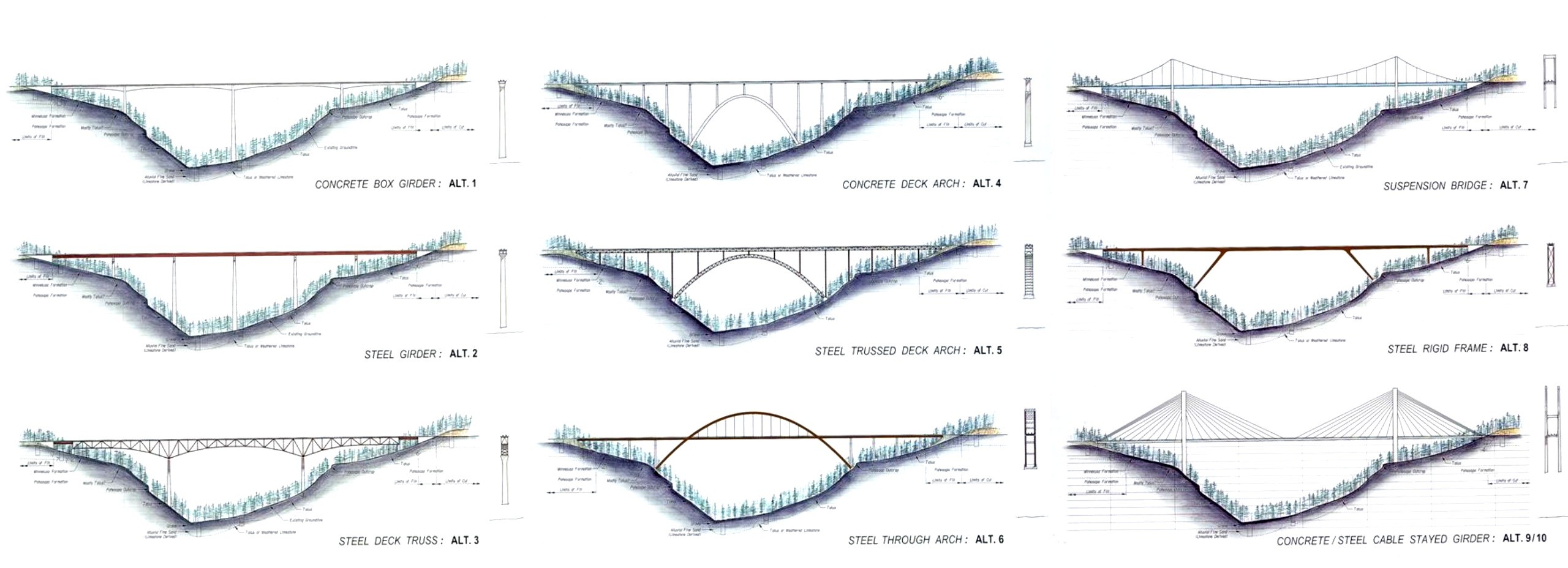
Options considered for the Hell Canyon crossing of US-16, South Dakota.
Depending on the span required, several different types of bridges are in common use today. Generally, short bridges (less than 100m span) are achievable via a concrete or steel beam construction. From 100m to 300m spans, truss or arch bridges become most economic, although segmental concrete types are still common. Cable-stayed bridges are optimal for spans from about 250m to 750m. Suspension bridges become economic at spans above 500m, with the largest constructed to date spanning almost 2000m. It is not known what the maximum possible span for a suspension bridge is, but there are currently plausible plans for bridges spanning up to 3km, and it is thought that 5km may be possible. It is of course possible to build a bridge comprising several lesser spans supported on pylons, but this becomes increasingly difficult in deep water, say, 50 metres or deeper (for example, the Golden Gate Bridge pylons sit in 30m of water). Additionally, it is often impractical to build bridge pylons in shifting riverbed sands or deep mud.
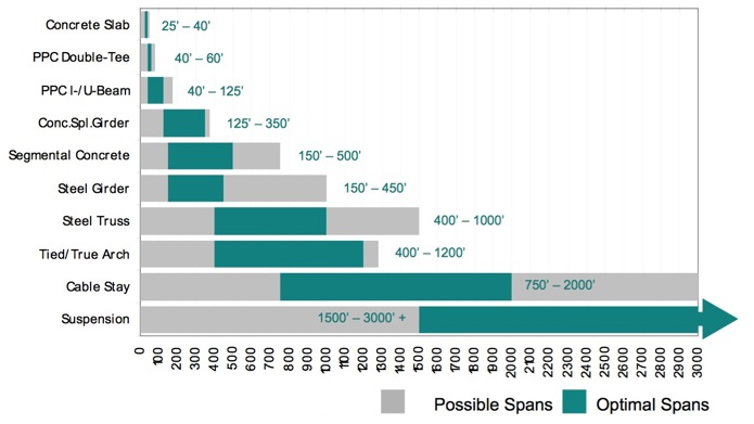
Bridge types and optimal span lengths in feet. Source: Portland-Milwaukie Light Rail Project
The construction cost of a bridge increases exponentially with increasing span, because the bending moment experienced by a bridge increases with the square of span. This results in an exponential cost function of the form:
Cost = AeBS
…where A and B are constants, and S is the bridge main span in metres. Different bridge types will have different values for A (the base coefficient) and B (the exponent coefficient). When we compare the different cost curves, we will obtain a graph of the following form:
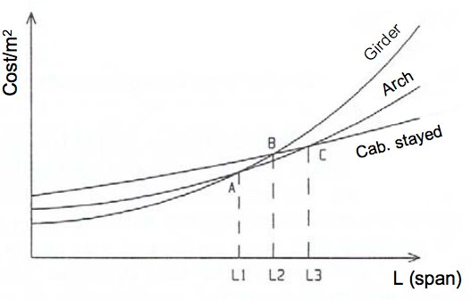
Relationship of bridge cost to main span. Source: Province of Bergamo, Italy.
Note that as span increases, the lowest cost bridge type shifts from girder, to arch, to cable stayed. The economic lengths L1, L2 and L3 correspond to the “optimal spans” of Figure 2. In order to roughly estimate bridge construction cost, we must find the equation of the cost curves.
Methodology
An internet survey of the various bridge classes was conducted. Bridges were identified using Wikipedia, Structurae, various bridge engineering textbooks and Google search. Data collected included construction cost, longest span, total length and number of lanes. If the year of construction cost was not stated, it was assumed to refer to the year of completion.
Nominal local currency was converted to 2013 US Dollars by first converting to US dollars in the year of completion, and then correcting for inflation. Exchange rates and CPI data are taken from www.measuringworth.com, while construction cost indices have been obtained from a variety of sources (see below). As the most recent year for which full-year data was available, the year 2013 was chosen as the reference year.
For bridges constructed after 1970, construction costs were adjusted by regional cost multipliers based on a 2012 comparative survey by EC Harris. Although this data refers specifically to 2012, it was assumed to apply to all bridges built since 1970. Bridges built prior to 1970 were assigned a regional multiplier of 1.
Cost was divided by number of lanes and total length to find a cost per lane-metre, and then plotted against main span length using Microsoft Excel. Although rail bridges are usually more expensive, a rail track was considered equivalent to a road lane, as this results in the most conservative estimate (ie highest cost). Bridges that had unduly long approach spans (such as the very long Øresund Bridge linking Denmark and Sweden) were excluded, unless a cost for the main bridge span itself, separate to the approach spans, was reported.
A cost function of the form Cost = AeBS was derived using Excel’s built-in trendline function. Values for A and B were recorded, as well as R2.
Limitations
The available cost data usually referred to the bridge project as a whole, which often included approach spans, on-ramps, road surface or rail track, and sometimes tunnels or second bridges. For example, the eastern span of the Great Belt Bridge is the third-longest suspension bridge in the world. Its Wikipedia article gives the 1998 construction cost as DKK21.4 billion (US$5.85 billion). However, this figure actually includes the cost of the East Bridge, the West Bridge, and the tunnel, as well as approach spans. The cost of the East Bridge alone is reported later in the article as US$950 million (1998 prices), less than a sixth of the total cost of the Great Belt Bridge project. For this reason, data was only included where it was reasonably certain that the reported cost referred to only the primary bridge structure.
Approach spans were treated as part of the overall length of the bridge unless a cost could be found for the main bridge structure alone (preferred), or eliminated from consideration if the approach spans were unduly long. Data were excluded where the total length was greater than 500% of the main span (unless the bridge consisted of multiple similar spans). Road surface and rail track was ignored (such cost is generally under $1000 per lane-metre, and thus a small proportion of total bridge cost).
Outliers were not generally removed, as it was considered that the possibility of cost blowouts should be reflected in the cost function. However, in extreme cases, it was concluded that the cost data was unreliable, and the data was excluded.
The use of 2012 regional cost comparison data to adjust bridge construction costs back to 1970 is a sub-optimal strategy. It would be preferable to use regional cost comparison data for each relevant year. However, the difficulty in finding such data rendered this strategy impractical. In any case, comparison with EC Harris studies from previous years suggested that the general cost differences between regions have remained fairly consistent since at least the 1990s. Additionally, the developed world (where most bridges in the survey are located) generally has a multiplier of around 1; most bridges in the survey built before 1970 are located either in the USA or UK, both of which have a multiplier of 1. Therefore although this method is flawed, it is considered superior to unadjusted data.
Accounting for inflation
In order to obtain a large enough sample of bridges for such a study, and to include the largest of certain spans, many of the surveyed bridges are quite old – in several cases over a century. It is critical to accurately account for the changes in construction prices over time; this incorporates materials cost, labour, and changing building regulations among other things, and the commonly-used Consumer Price Index (CPI) is not generally a good proxy for construction costs.
There are several commonly used construction indices, however they generally do not extend back as far as we require. The California Department of Transport has exactly the kind of index we need – a bridge construction cost index. However, it only extends back to 1966, limiting its usefulness. We could simply eliminate any bridge built before 1966, but this would severely restrict the sample size of deck-arch and truss type bridges. Additionally, it is limited to prices in the state of California, resulting in a very high volatility, making this index inappropriate for analysing a worldwide sample.
One of the most well known and longest-lived construction indices is the Construction Cost Index published by the American magazine Engineering News Record, which has data as far back as 1908. It is calculated by tracking the prices of a limited basket of goods: unskilled labour, cement and lumber. ENR started publishing a second index in 1920, the Building Cost Index, which substitutes skilled labour for unskilled. Both indices continue unbroken to the present day. Critically, they encompass the drastic labour market upheavals caused by both world wars. However, this limited basket of goods is not specific to bridge construction.
Another common and well-respected index is the US Army Corps of Engineers Civil Works Construction Cost Index (CWCCI), using data drawn from all 50 US states. The CWCCI is a weighted average of 20 individual cost indices for various classes of civil engineering projects, one of which is “Roads, railroads and bridges” – this is perfect, however the data only extends back to 1967.
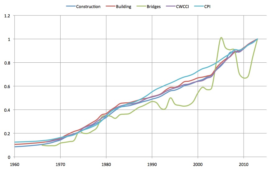
Various cost indices since 1960 (Base year 2013 = 1)
It was chosen to construct a hybrid index using the CWCCI index for roads, railroads and bridges from 1967-2013, an average of the the ENR Construction Cost Index and Building Cost Index from 1908-1966, and the USA Consumer Price Index for all years prior to 1908. The three indices were merged into a single index by normalising at each transition year. The BCI and CCI were averaged as the CWCCI tracks between the two of them for most of the period 1967-2013. This method was found to produce the highest average coefficient of determination, and resulted in highly plausible results for economic span.
Results
Beam
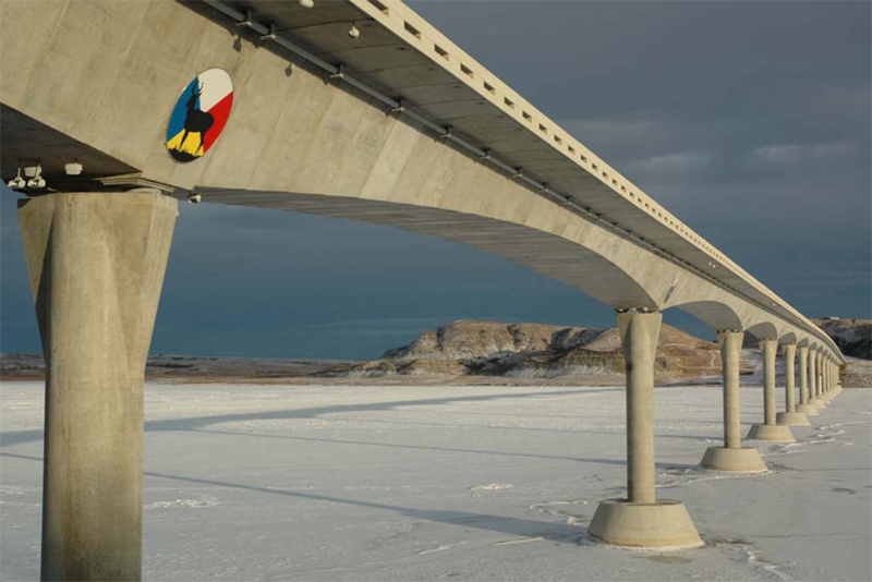
Four Bears Bridge, North Dakota.
A “beam bridge”, for the purposes of this study, includes several different types of bridge characterised by being comprised of a relatively simple “beam” or “girder” construction, whether simply supported, hinged or cantilevered (but not including truss-cantilevered). The span of such bridges varies extremely widely, from under 10m for the simplest concrete slab bridges, to over 300m for the largest of balanced-cantilever segmental concrete construction.
The vast majority of bridge structures worldwide are of the beam type, mostly of relatively short span and not generally notable enough to warrant a Wikipedia article. On the other hand, the sheer number of such spans makes it fairly simple to find a sufficient number of empirical examples.
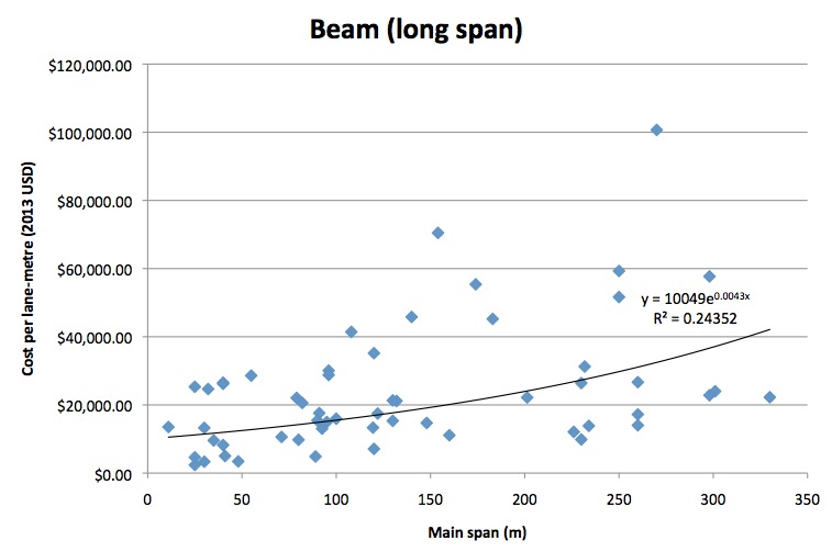
Sample size was 56, with median year of construction 1997. Span ranged from 11m to 330m, with a median of 120m. The cost-function coefficients were A=10049, B=0.0043, with R2 of 24.4%.
Generic, short-span bridges
As noted above, the vast majority of bridges are of a beam type with a span of under 100m. However they are underrepresented in our data. We can address this by including existing cost estimation models for various types of short-span beam and girder bridges.
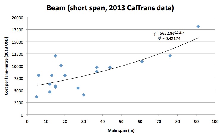
The California Department of Transport gives typical span and cost-per-square-metre ranges for different types of beam bridge over the last decade. High and low estimates are given for both span and cost; low cost was assumed to correspond to low span, and vice versa, thus obtaining two datapoints for each bridge type.
To convert these area costs into cost per lane-metre, the average dimensions of a bridge must be known. US Interstate highway standards stipulate that a bridge must have minimum 12-foot (3.7 m) lanes with 10-foot (3.0 m) outside and 3.5-foot (1.1 m) inside shoulders. Including shoulders, the average width of a bridge comes to about 5 metres per lane. However, not all bridges are highway-grade and would have narrower shoulders, and often no central shoulder at all. Additionally, many jurisdictions allow relaxed standards for bridge verge widths, on account of those structures’ great expense. A typical width per lane of 4m was assumed.
The cost function coefficients were found to be A=5652.8, B=0.0113, with R2 of 42.2%.
Truss
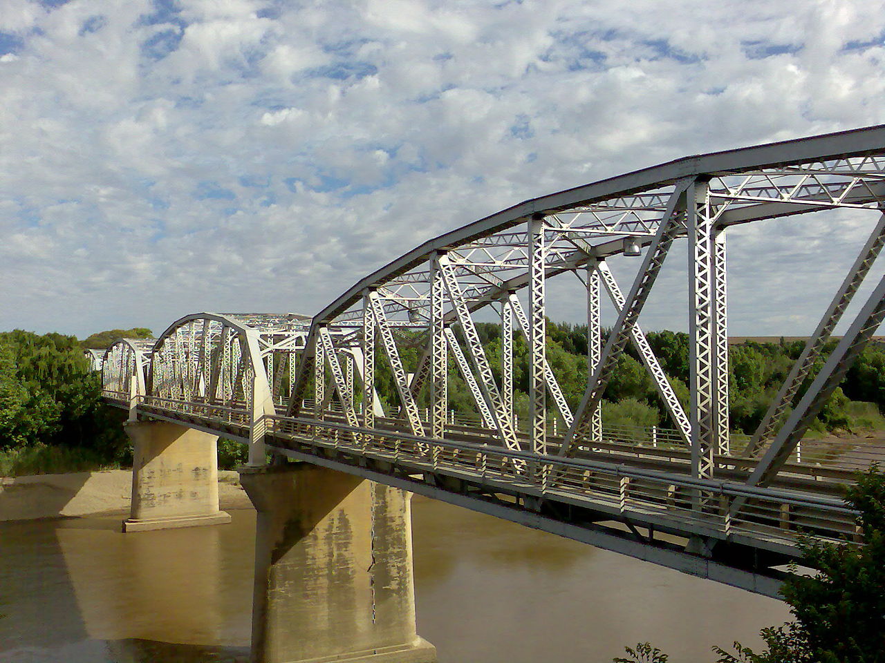
General Hertzog Bridge, South Africa.
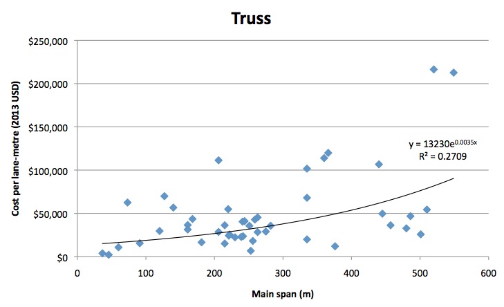
The truss bridge is a structure of connected elements forming triangular units. The study includes simple trusses such as Warren, Allen or Pratt trusses (shown above) in this category, as well as the more complex cantilever truss bridge (the pre-eminent example of such being the Forth Bridge in Scotland). They are generally obsolete, having been surpassed in technology by the beam bridge, and later the cable-stayed bridge for longer spans. However they are still built occasionally where the specific features of the project are best served by such a type. The sample size was 47, with a relatively old median year of construction at 1958. Span ranged from 37m to 549m, with a median of 242m. The cost-function coefficients were A=13230, B=0.0035, with R2 of 27.1%.
Deck-arch
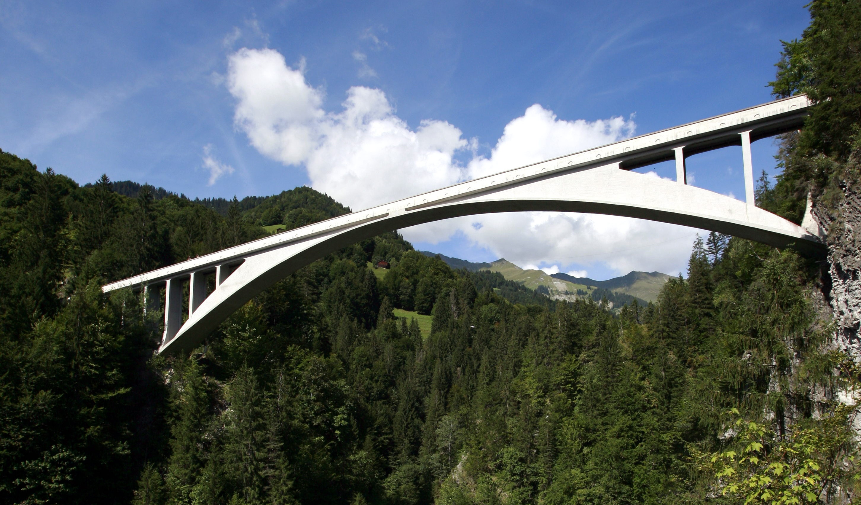
Salginatobel Bridge, Switzerland.
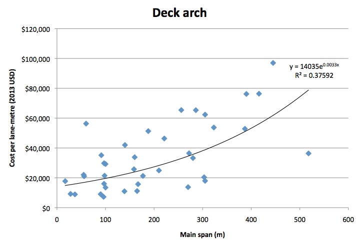
Also known as the “true arch”, the deck-arch bridge is arguably the most aesthetically pleasing bridge type. It works by transforming the loads partially into a horizontal thrust force, which is resisted by abutments (bridge foundations) at either end of the arch curve. For this reason, as well as restrictions imposed by geometry, the type is particularly suited to construction in deep valleys or ravines. Despite being relatively expensive per lane-metre, the deck-arch bridge can often be economic due to its particular appropriateness to construction in deep valleys; the abutments can often be far closer together than the ends of the road deck, resulting in a shorter main span than other bridge types would be able to achieve (for illustration, see the diagrams of potential designs for the Hell Canyon bridge in South Dakota, at the beginning of this article). Additionally, they are usually constructed with no approach spans, resulting in a relatively short total length. The sample size was 39, with median year of construction 1963. Span ranged from 17m to 518m, with a median of 167m. The cost-function coefficients were A=14035, B=.0033, with R2 of 37.6%.
Through- or Tied-arch
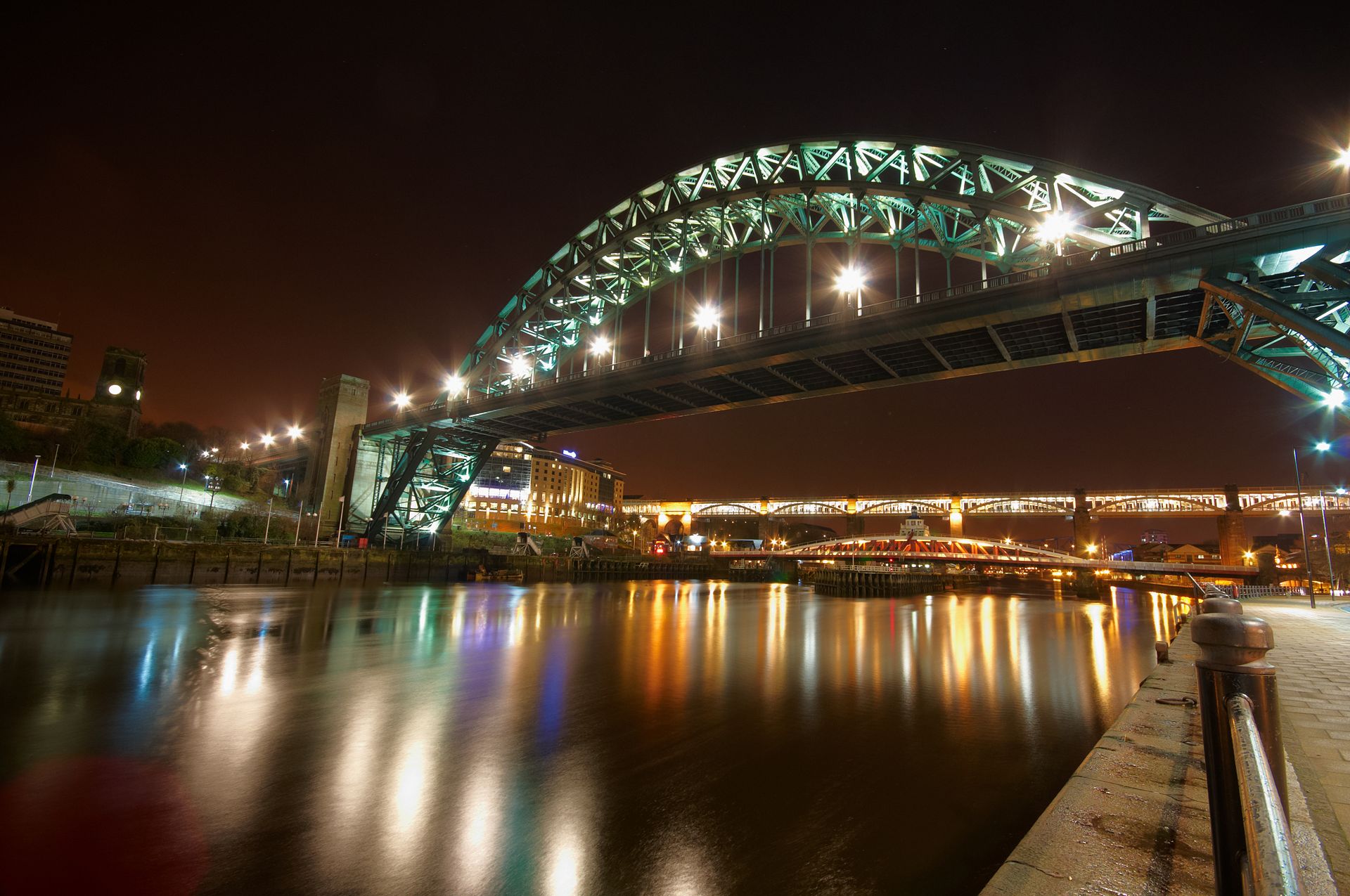
Tyne Bridge, England.
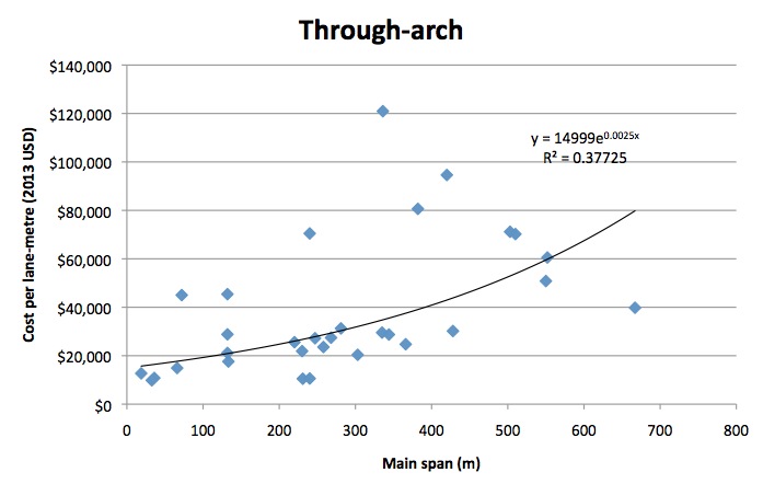
Although structurally different, the through-arch bridge and the tied arch bridge are included in the same category due to being functionally similar (having the deck below the arch), and thus being appropriate for similar geographic locations (unlike the deck-arch, which requires a deep valley). The through-arch transfers the load of the suspended deck to compressive forces in the arch, which are then transferred to the earth via the abutments. By contrast, the tied-arch bridge restrains the ends of the arch through tension forces in the deck structure itself, in the manner of a bowstring. Sample size was 31, with median year of construction 1978. Span ranged from 19m to 667m (the largest span being still under construction), with a median of 258m. The cost-function coefficients were A=14999, B=.0025, with R2 of 37.7%.
Cable-Stayed
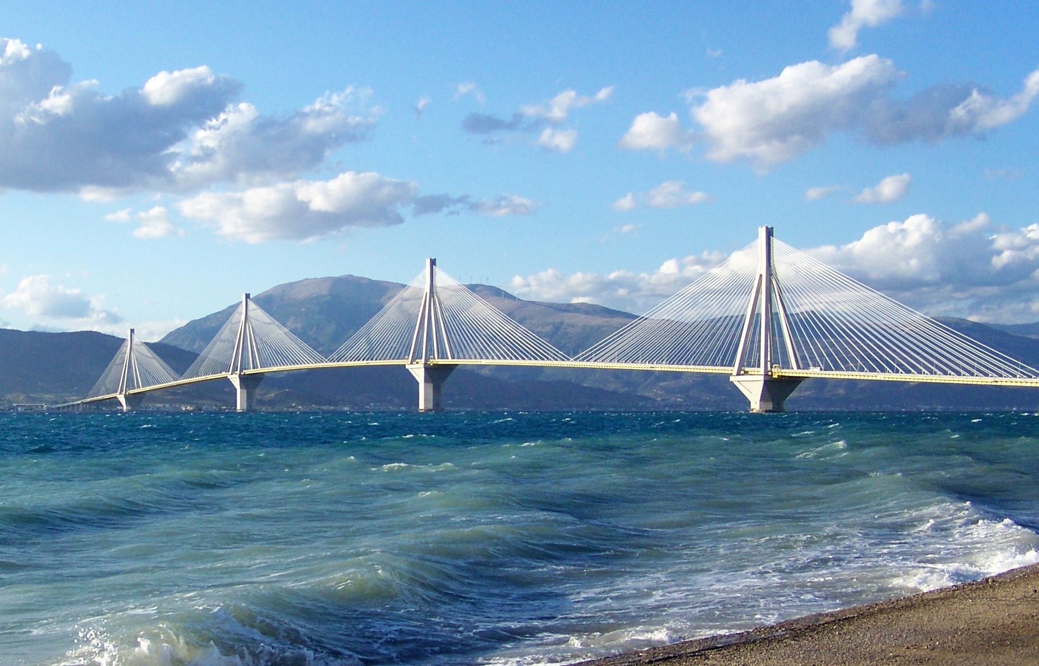
Rio Antirio bridge, Greece
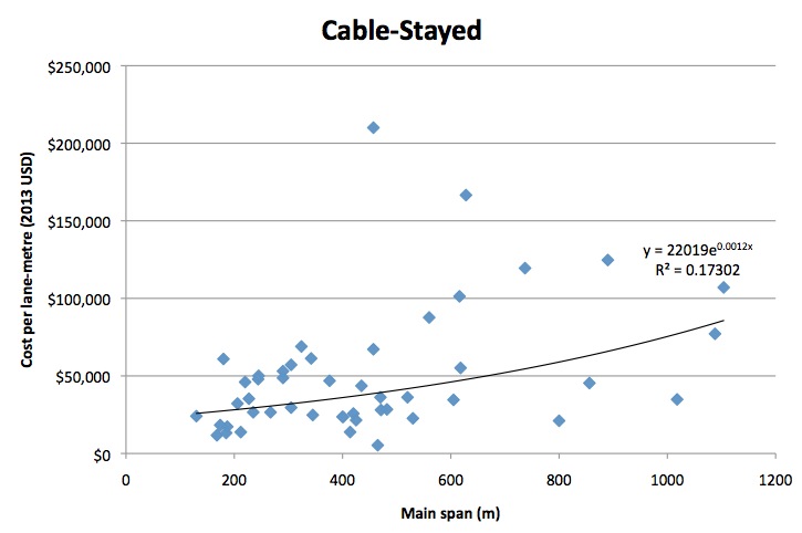
Although superficially similar in appearance to a suspension bridge, the cable-stayed bridge is structurally very different. The deck is commonly of segmental concrete, with the “stays” supporting the deck from one or more towers. The tension loads in the cables are transferred into compressive loads in the tower(s), which hold the entire weight of the bridge (thus unlike suspension bridges, they can be built with a single tower, although this is uncommon). Sample size was 48. This was the youngest class of bridge, with a median construction year of 2004. Span ranged from 130m to 1104m, with a median of 408m. The cost-function coefficients were A=22019, B=.0012, with R2 of 17.3%.
Suspension
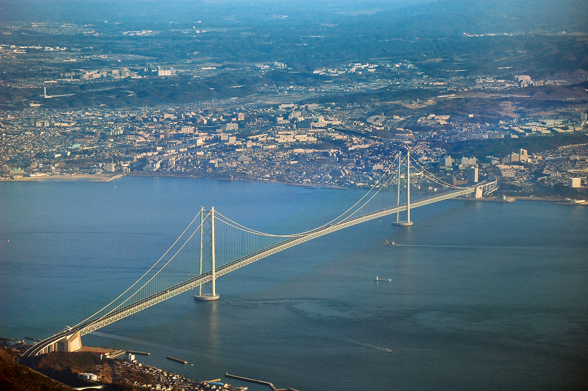
Akashi Kaikyō bridge, Japan.
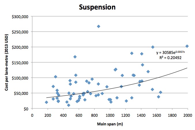
Suspension bridges are the longest class of bridge; the largest existing span is the 1991m of the Akashi Kaikyō Bridge in Japan (shown above). They work by transferring the load of the deck into tension forces in the suspension cables. These cables are slung across two or more pylons, with the tension forces resisted by anchorages at either end. Sample size was 64, with a median construction year of 1988. Span ranged from 182m to 1991m, with a median of 730m. The cost-function coefficients were A=30585, B=.0007, with R2 of 20.5%.
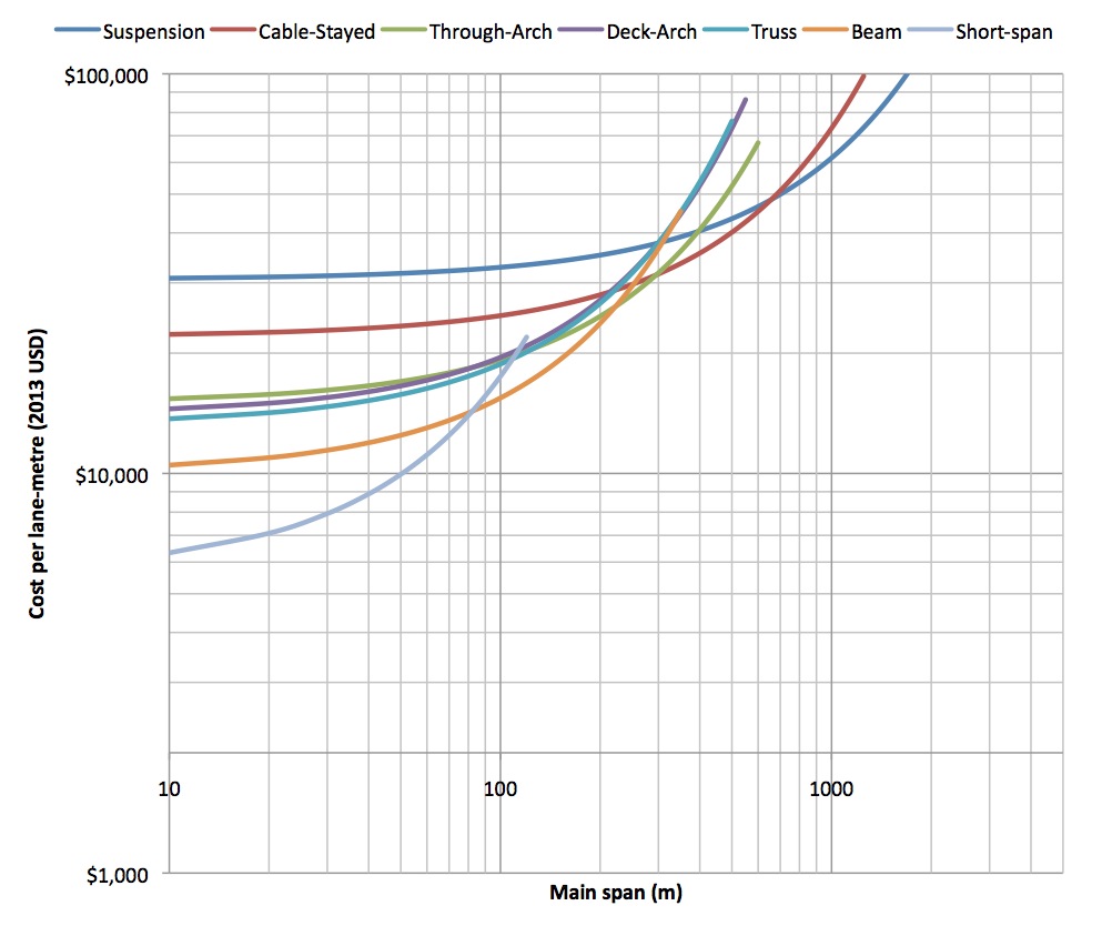
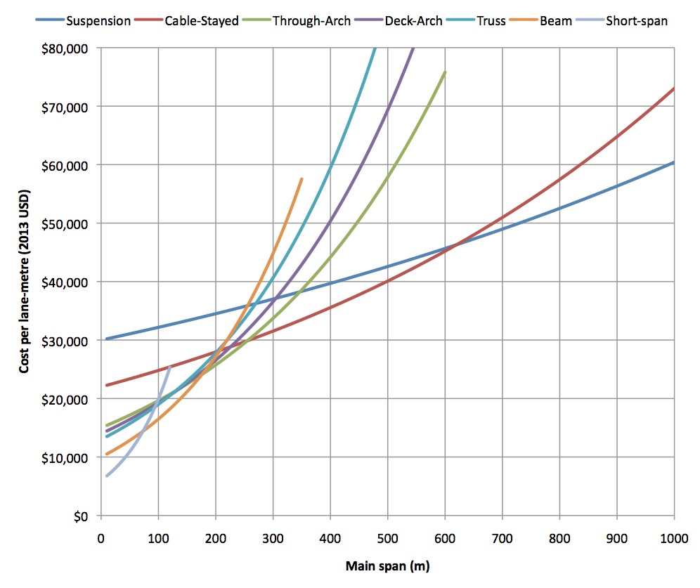
Summary
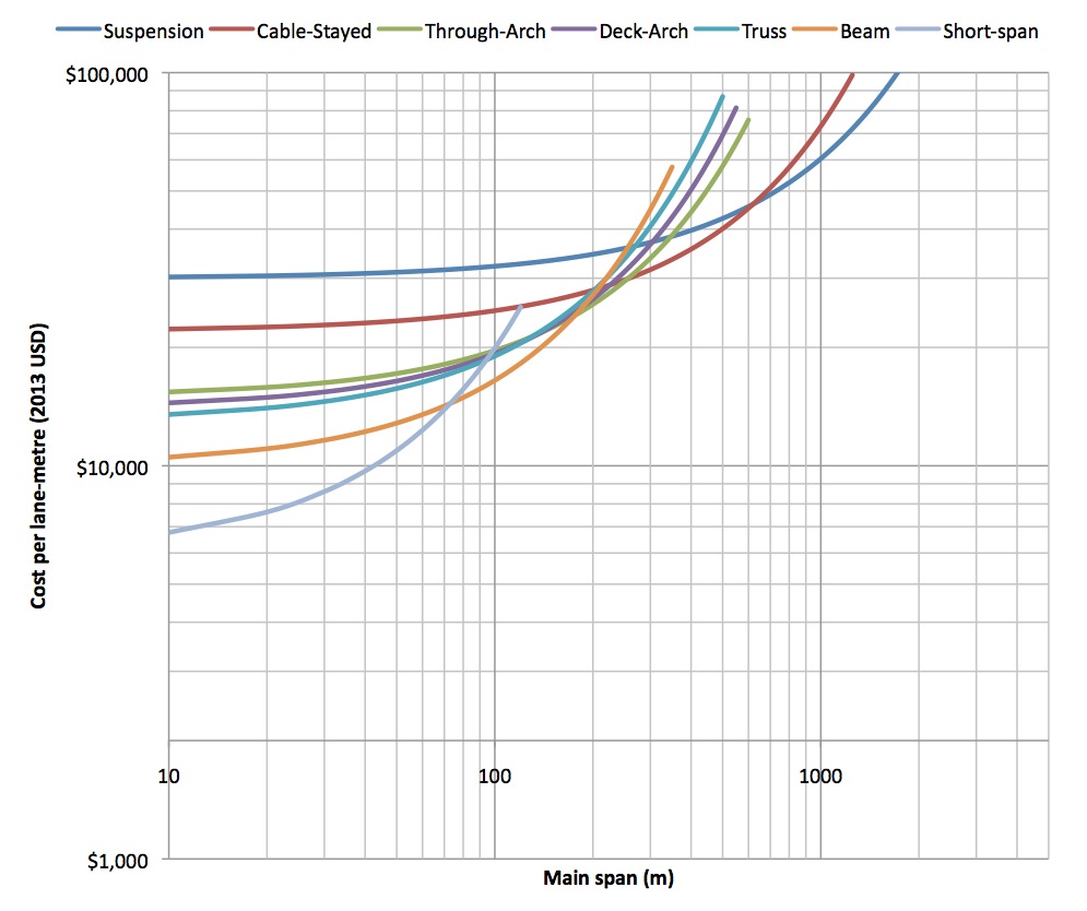
The cost functions derived for each bridge type are plotted together in the following figures, first on a linear scale, and subsequently on a log scale to better view the relationships at shorter spans: 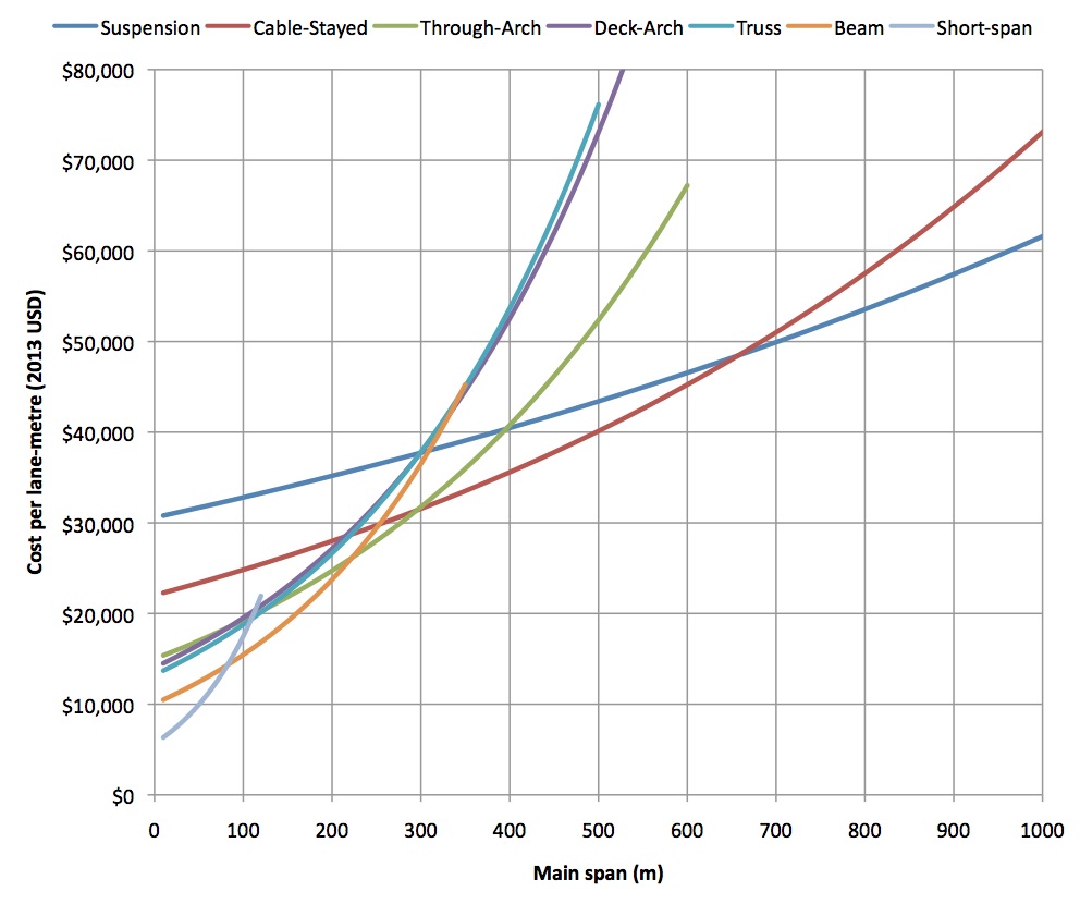
Discussion
The results were remarkably close to the expected economic spans:
- Short span beam bridges were the most economic choice until approximately 80m
- Longer segmental concrete and steel girder beam bridges were the most economic choice until a little over 200m; this is substantially greater than the 130m expected, and possibly reflects the improved construction techniques in segmental concrete bridge construction in recent years.
- Truss and arch bridges each become economic at spans slightly longer than 100m (although only through-arch ever overtakes segmental concrete).
- Cable-stayed bridges become economic at spans above 300m, slightly greater than the expected 250m.
- Suspension bridges become economic at spans over 650m, substantially greater than the expected 500m. This possibly reflects recent improvements in cable-stayed construction.
Coefficient of Determination ranged from 17% to 37%, indicating that between 63%-83% of the variation in costs is not explained by the cost function. This is as expected; every bridge has unique engineering requirements, including but not limited to load characteristics, foundation type, corrosion environment, seismic conditions, height of pylons, depth of cassions, proximity to other development, accidents and many others. It is also likely that some of the error stems from the inconsistent use of regional multipliers.
Given the inherent uncertainty in the particular data, but assuming that the trends are broadly consistent with future construction costs, we can propose minor modifications to the values of A and B (slightly upward or negligible) in order to better reproduce the observed economic spans and trends, and also to maximise the usefulness of the cost functions as a tool for comparison between different design options. The proposed model adjustments are shown below:
[table]
Bridge type, A (data),B (data),A (modified),B (modified)
Beam (short),5652.8,0.0113,6000,0.012
Beam (long),10049,0.0043,10000,0.005
Truss,13230,0.0035,13000,0.0038
Deck-Arch,14035,0.0033,14000,0.0032
Through-Arch,14999,0.0025,15000,0.0027
Cable-Stayed,22019,0.0012,22000,0.0012
Suspension,30585,0.0007,30000,0.0007
[/table]
Using the cost functions
To estimate the cost of a particular bridge type:
- Determine the requirements of the bridge – traffic lanes, rail lanes, main span, total length, length of any approach spans
- Based on main span, find the cost per lane-metre using the appropriate cost function.
- Multiply by number of lanes, ensuring that any rail tracks are counted as 1.5 lanes.
- Multiply by total length (this will always be at least as long as the main span).
- Repeat steps 2-4 for any approach spans of a different type.
- Add total expense for main structure and approach spans.
- Multiply by regional modifier if applicable.
Side spans
Some bridge types, particularly cable-stayed and suspension bridges, must extend a certain distance beyond the main span due to the geometry of their design. For cable-stayed bridges, these “side spans” are each about 40%-50% of the main span; for suspension bridges, they are typically 20% to 25% of the main span, but may be as little as 0% (usually for very short bridges) or as much as 50%. Deck-arch bridges also typically extend beyond the main span, though the amount is highly geography dependent.
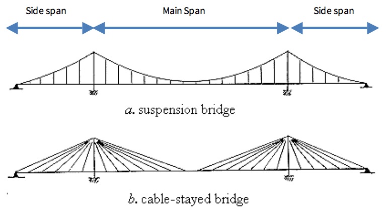
Examples of side spans. Source: Brigham Young University
Regional Multipliers
EC Harris released a report on comparative construction costs around the world in 2012. Using costs in the UK as a baseline, the following factors are applied for construction in other countries (average of range given to nearest 5%):
- Switzerland: 1.6
- Scandinavia: 1.4
- Australia: 1.35
- Japan: 1.3
- Canada: 1.15
- Western Europe: 1.1 (typical)
- USA: 1.00
- Russia: 0.85
- South Korea: 0.80
- Eastern Europe: 0.65 (typical)
- China: 0.50
- India: 0.25
Modal Multiplier
In this study, we have so far assumed each each road or rail lane to be equal (and ignored pedestrian and cycleways). However, dead, live and dynamic loadings are higher for rail than for road, especially HSR. According to guidelines used in the Spanish high-speed rail network, HSR bridges typically require design loadings 235% that of an equivalent road bridge due to the increased mass and speed of the vehicles. However, the source does not comment on the effect of this on cost. A 2006 British study by built asset consultancy EC Harris claimed that the cost per deck area of rail bridges was between 36% and 55% higher than for road bridges. Therefore, to use these cost functions for rail bridges or combination road-and-rail bridges, a rail track is equal to 1.5 “lanes”.
No data was found comparing pedestrian bridges to road bridges, but live loads are generally very small in comparison to dead loads. In the absence of any data whatsoever, a reasonable guess might be to apply a factor of 0.5 (referring to a shared two-way pedestrian/cycleway), or 0.25 per one-way pedestrian or cycle lane.
Short Bridge Multipliers
EC Harris also suggested that short bridges consisting of only a few spans were significantly more expensive than bridges of numerous spans. This is due to the fact that for short bridges the design and engineering costs become a substantial part of total bridge cost. For bridges of the “short span” type, apply the following multipliers:
[table]
Spans,Multiplier
1,2.35
2,1.67
3,1.15
4+,1.00
[/table]
Verification examples
The following examples shall give prices in United States construction equivalent, so step 7 (regional multiplier) will be skipped.
Anzac Bridge, Sydney
Let’s look at the cable-stayed Anzac Bridge in Sydney, Australia as a verification example, as it is a relatively recent construction, with well defined lengths and well verified cost data. The bridge has no approach spans, only side spans.
- Carries: 8 lanes of traffic, 1 shared cycleway
- Main span: 345m
- Total length: 805m
- Original construction cost: $170 million (1995 AUD)
- Regional multiplier: 1.35
- Adjusted construction cost: $159,644,000 (2013 USD inflated using CWCCI and adjusted for regional differences)
It is a cable-stayed bridge with main span of 345m, therefore our cost function is 22,000e(0.0012×345), which equals $33,283 per lane-metre. The bridge has 8 traffic lanes, plus one cycleway with a multiplier of 0.5, which adds up to 8.5 lanes equivalent. Now multiply the cost function by the number of lanes and the total length:
$33,283 × 8.5 × 805
= $227,738,000 (nearest $1000)
In this case, the cost function has over-estimated the actual cost by 42.7%. However, this is largely due to the weak Australian dollar of 1995 causing an underestimate of the adjusted construction cost. If the Australian dollar had been at or near parity with the US dollar (as it has been in recent years), the estimate would have been substantially closer. At any rate, the result is adequate for a ROM costing, and well within the expected error for cable-stayed bridges, as indicated by the R2 values.
How about another one, a bit more complex this time?
Chaotianmen Bridge, China
Currently the largest through-arch bridge in the world, the Chaotianmen Bridge in Chonqing, China, has six traffic lanes and two pedestrian lanes on its upper deck, and two traffic lanes and two rail tracks on its lower deck. The main span is 552m, the total length is 1741m, but the bridge is actually of two parts: the main structure is of a through-arch construction; analysis of Google Earth imagery shows it to be 948m long. That leaves 973m of approach spans of a simple beam construction, with a span of 45m (again determined by Google Earth imagery).
- Number of lanes: 8 traffic + 2 rail (1.5 each) + 2 pedestrian (0.25 each) = 11.5 lane-equivalent
- Original construction cost: 3.25 billion Yuan (2009)
- Regional multiplier: 0.5
- Adjusted construction cost: $1,054,116,000 (2013 CWCCI-adjusted USD)
We do this in two parts: first the main structure. Through arch with span of 552m gives a cost function of 15000e(0.0027×552), coming to $66,583 per lane-metre. Multiplying by number of lanes (11.5) and length of structure in metres (950), this gives us a USA-equivalent construction cost for the section of $727,420,000.
Second, the approach spans. These spans are short-span beam construction, longest span 45m, therefore the cost function is 6000e(0.012×45), which comes to $10,296/lane-metre. Multiply by (11.5 x 973) gives a section cost of $115,208,000
Therefore the total cost of the bridge is the sum of approach spans and main span, being $842,628,000. This is an underestimate of 20%, but still, a decent first estimate.
Future work
Although the results closely reproduced the expected economic spans, substantial uncertainty remains. Future work should focus on applying appropriate regional multipliers for each year. This data may be hard to come by, and it may be necessary to restrict the contents of the survey to bridges from the developed world, especially for older bridges. For this to be a suitable outcome, the sample size would have to be greatly increased. This would likely require much more detailed research, using source documents not easily obtainable over the internet.
Accounting for seismic loading, wind loading and pylon height/depth would also allow the cost functions to more accurately estimate a wide range of construction scenarios.
Data
The data for the bridge survey, inflation and foreign exchange are available in the following Excel spreadsheet: